Tracers

Tracers provide an agnostic interface to implement logging, reporting, and real-time monitoring of the annealing process. They allow you to “hook” into each iteration of the algorithm to capture the current state without modifying the core logic of the optimization.

Definition

A tracer is defined as a callable that accepts the current AnnealingState and returns nothing. In the core implementation, it follows this type alias:

type Tracer[T] = Callable[[AnnealingState[T]], None]

Usage

To use a tracer, you assign it to the tracer property of a SimulatedAnnealing instance. By default, the algorithm uses a no-op tracer (_no_trace) which does nothing.

Function-Based Tracers

For simple logging or printing, a plain function is often sufficient:

def simple_logger(state):
    if state.iteration % 100 == 0:
        print(f"Iteration {state.iteration}: Best Value = {state.best_value}")

sa = SimulatedAnnealing(...)
sa.tracer = simple_logger
sa.simulate(initial_state)

Object-Based Tracers

For more complex scenarios, such as accumulating data into a data structure or generating plots, you can implement a tracer as a class with a __call__ method. This allows the tracer to maintain its own internal state across iterations.

Example: A simple history accumulator:

class HistoryTracer:
    def __init__(self):
        self.history = []

    def __call__(self, state):
        # Store a copy of the current best value
        self.history.append(state.best_value)

history_tracer = HistoryTracer()
sa.tracer = history_tracer
sa.simulate(...)

print(f"Captured {len(history_tracer.history)} data points.")

Customization

Since tracers are agnostic, you can easily wrap existing logging libraries (like loguru or standard logging) or even send metrics to external services like Weights & Biases or MLflow by simply implementing the tracer interface.

DataFrameTracer

The DataFrameTracer is a powerful tool for post-optimization analysis. It records the state of the annealing process at specified intervals and converts the history into a pandas.DataFrame.

This tracer is particularly useful when you want to visualize the convergence, analyze the exploration of the search space, or export the run data for external tools.

Basic Usage

To use the DataFrameTracer, initialize it and assign it to your SimulatedAnnealing instance. After the simulation is complete, you can access the accumulated data via the frame property.

from altbacken.internal.tracer.dataframe import DataFrameTracer

# Initialize the tracer
tracer = DataFrameTracer(frequency=10)
sa.tracer = tracer

# Run the simulation
best_sol, best_val = sa.simulate(initial_guess)

# Access the results as a DataFrame
df = tracer.frame
print(df.head())

Recording Frequency

The frequency parameter controls how often the state is recorded. A frequency of 1 (default) records every iteration. For long-running optimizations with thousands of iterations, increasing the frequency (e.g., to 10 or 100) helps manage memory usage and improves performance of subsequent analysis.

Naming Schemes

When the solution space is a sequence (like a list of coordinates), DataFrameTracer automatically flattens these into individual columns. You can control the column names using the naming_scheme parameter:

Template String: Uses a format string (default is "x_{}").

tracer = DataFrameTracer(naming_scheme="coord_{}")
# Columns will be coord_0, coord_1, ...

Iterable of Strings: Uses a fixed list of names.

tracer = DataFrameTracer(naming_scheme=["latitude", "longitude"])
# Columns will be latitude, longitude

The resulting DataFrame will contain: * Flattened coordinates for the current solution. * Flattened coordinates for the best solution found so far (prefixed with best_). * Standard state fields: iteration, temperature, current_value, best_value, and improvement.

Properties

frame: Returns a pandas.DataFrame containing all recorded iterations.
coordinates: Returns a list of the column names used for the solution dimensions.
naming_scheme: Allows getting or setting the naming strategy used for columns.

ShowcasePlot

The ShowcasePlot is a high-level visualization tracer that builds upon the DataFrameTracer. It simplifies the process of creating comprehensive visual reports of the optimization run, showing how the algorithm explores the space and how the fitness value evolves over different phases.

Basic Usage

To use ShowcasePlot, set it as your tracer during the simulation. Once the simulation is finished, call the plot() method to generate a multi-panel visualization.

from altbacken.external.tracer.plot import ShowcasePlot

# Initialize the showcase plot
showcase = ShowcasePlot(frequency=5)
sa.tracer = showcase

# Run simulation
sa.simulate(initial_state)

# Generate and display the plot
p = showcase.plot()
p.show()

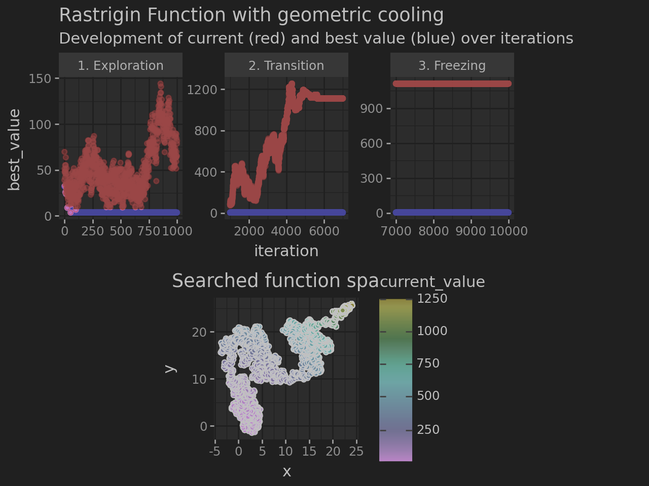
Visualization Components

The generated plot includes several sections:

Phase Plots: Visualizes the current_value and best_value across different stages of the process (Exploration, Transition, Freezing).
Exploration Plot: Shows a 2D density map of the explored function space for every combination of coordinates.
Temperature Plot: Displays the cooling schedule over time.

Customization

You can customize the appearance and behavior of the plots:

Colormap: Change the color scale used for temperature and values.
```
showcase.colormap = "viridis"
```
Y-Axis Scaling: Control whether facets share the same Y-axis scale.
```
showcase.free_y_axis = False  # Force shared Y-axis
```
Phase Labeling: By default, iterations are split into three equal phases. You can provide a custom

PhaseLabeler to the plot() method to define custom phase logic.

The PhaseLabeler deduces the phase label from the DataFrame as Series and is defined as

type PhaseLabeler = Callable[[DataFrame], Series[str]]

it could be used to define the label by temperature like:

def by_temperature(df: DataFrame) -> Series[str]:
    return df.temperature.map(lambda x: 'Cold' if x < 1000 else 'Hot')

Plot Size: Adjust the output dimensions.

# Output a 10x15 inch plot
p = showcase.plot(size=(10, 15))

Dependencies

This tracer requires the plotnine and pandas libraries to be installed.