Graph Example

In this example we try to find a graph that represents a network of pipelines with a flow of water. The goal is to find a graph that has a total flow of 5 units and no isolated nodes. The fitness function is designed to penalize graphs that have a dissipation of flow, isolated nodes, or a total flow that is not 5 units.

from networkx import (
    Graph, DiGraph, draw_networkx_edges, draw_networkx_nodes,
    get_edge_attributes, draw_networkx_edge_labels, circular_layout
)

from altbacken.core.annealing import RandomChoice
from altbacken.external.annealing import SimpleSimulatedAnnealing
from altbacken.external.neighbourhood.graph import GraphNeighbourhood, AddNode, AddEdge, RemoveNode, RemoveEdge
from altbacken.external.temperature import LogarithmicCooling

Alter flow modification

We introduce a modification that allows us to alter the flow of a pipeline. This modification is used to explore the space of possible solutions by changing the flow of a pipeline.

def alter_flow(graph: Graph, *, choice: RandomChoice) -> bool:
    if not graph.edges:
        return False
    edge = choice(list(graph.edges))
    flow: int = max(1, graph.edges[edge]['flow'] + choice([-1, 1]))
    if flow == graph.edges[edge]['flow']:
        return False
    else:
        graph.edges[edge]['flow'] = flow
    return True

Neighbourhood

We set the neighbourhood for the graph. The neighbourhood defines the set of modifications that can be applied to the graph. In this case, we have modifications for adding nodes, adding edges, removing nodes, removing edges, and altering the flow of a pipeline.

neighbourhood: GraphNeighbourhood = GraphNeighbourhood(
    modifications={
        AddNode(): 3,
        AddEdge({"flow": 1}): 3,
        RemoveNode(): 1,
        RemoveEdge(): 1,
        alter_flow: 5
    }
)

Fitness Function

The fitness function consists of three components: dissipation, overall flow, and isolated nodes. Dissipation is the sum of the absolute values of the overflow at each node. Overall flow is the sum of the flow of all edges. Isolated nodes are nodes with no edges connected to them. Overall flow and dissipation pull in different directions. We want to minimize dissipation and maximize overall flow. Isolated nodes are penalized. Overall flow and dissipation pull in different directions. We want to minimize dissipation and maximize overall flow. Isolated nodes are penalized.

def calc_dissipation(graph: DiGraph) -> float:
    value: int = 0
    for node in graph.nodes:
        overflow: int = 0
        for edge in graph.in_edges(node):
            overflow += graph.edges[edge]['flow']
        for edge in graph.out_edges(node):
            overflow -= graph.edges[edge]['flow']
        value += abs(overflow)
    return value

def calc_overall_flow(graph: DiGraph) -> int:
    value: int = 0
    for edge in graph.edges:
        value += graph.edges[edge]['flow']
    return value

DESIRED_FLOW: int = 10
DESIRED_NODES: int = 5

def fitness(graph: DiGraph) -> float:
    dissipation: float = calc_dissipation(graph)
    overall_flow: int = calc_overall_flow(graph)
    isolated_nodes: int = sum(1 for node in graph.nodes if graph.degree(node) == 0)
    return dissipation + max(0, DESIRED_FLOW - overall_flow) + isolated_nodes + max(0, DESIRED_NODES - len(graph.nodes))

Simulation

We simulate with a logarithmic cooling scheme. Feel free to try other cooling schemes or play with the temperature

annealing: SimpleSimulatedAnnealing = SimpleSimulatedAnnealing(fitness, neighbourhood, LogarithmicCooling(100000))
best, score = annealing.simulate(DiGraph())
print("Fitness       : ", score)
print("Dissipation   : ", calc_dissipation(best))
print("Overall Flow  : ", calc_overall_flow(best), f"(expected min {DESIRED_FLOW})")
print("Nodes         : ", len(best.nodes), f"(expected min {DESIRED_NODES})")
print("Isolated nodes: ", sum(1 for node in best.nodes if best.degree(node) == 0))

Fitness       :  7
Dissipation   :  4
Overall Flow  :  8 (expected min 10)
Nodes         :  5 (expected min 5)
Isolated nodes:  1

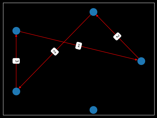
Visualization

Next we draw the graph. The fitness is non-smooth, multi-objective, and mixes hard constraints (conservation) with soft ones (minimum flow, minimum nodes). Despite that, SA still trends toward reasonable graphs because local changes usually affect fitness in a consistent direction, and temperature helps jump out of traps

pos = circular_layout(best)
draw_networkx_nodes(best, pos)
draw_networkx_edges(best, pos, edge_color="red", arrows=True)
draw_networkx_edge_labels(best, pos, edge_labels=get_edge_attributes(best, "flow"))

{(1, 2): Text(0.6545134471069989, 0.47552144216518943, '2'),
 (2, 5): Text(-0.2500001438200925, 0.18163545643614243, '2'),
 (3, 1): Text(0.0954942171513593, 0.2938917387184805, '1'),
 (5, 3): Text(-0.8090170266926682, -9.259401781980259e-06, '3')}